An Introduction to OpenLayers 3, Part II

Last week, we created a basic web map by loading a basemap from OpenStreetMap using OpenLayers 3 (OL3).  If you missed last week's post, below are links to the code:

• Click to view the text file
• Click for the HTML file 

This week I will cover copying OL3's JavaScript libraries to a web hosting service. Also, note that you can run basic OpenLayers code off your computer--it simply depends on where the sources of data are located and how the code is written.

In order to get your map visible on the web, you will need a web hosting service or your own server.  After setting up an account, you will have a chance to upload files. Before that, there are a few things you need to know:

• You will upload folders and files from the OL3 JavaScript library to the public or root directory of your web hosting service.  
• In some cases, this is simply a matter of placing files in a folder; for some services you may have to set permission levels to public/everyone.
• An additional step for uploading and accessing layers.
•  In the next post, we will upload, use, and symbolize this uploaded layer.  
• OL3 runs client-side (vs the server) so keep that in mind, so you won't want to use this method for large layers.
• You don't need to do this step or the next one if you are accessing layers using a web map service or WMS.
• Later I will also look at using GeoServer for more complex layers.
• In addition, you will have to create a simple web config file to access files on your web hosting service. 
• This can be done in a text editor, like Notepad. 
• For example if you plan to use KML files, you will have upload a file with the following code for particular media or MIME types. 
• Click to magnify the screenshot below for an example for a *.kml file.

You can find code for other MIME types by searching the web.
Save this code as web.config and upload to the root directory of your web hosting service.

After downloading and unpacking the *.zip file from OL3 (or OL2), you will see several folders and files. 

• Consider copying all the folders and files over to see examples and understand how the code works
• Keep in mind how you copy folders and files over, since this will affect how you write code and reference directories.
• Lastly, the ol.js file you need is in the build folder.  In the first example that I showed (in the code above), you need to change the link to the OL3 website from "http://ol3js.org/en/master/build/ol.js" to "build/ol.js."  The same goes for the css stylesheet.

Next time, we will look at uploading, using, and symbolizing a KML.

For serious developers, be sure to check out the OL3 wiki at: https://github.com/openlayers/ol3/wiki

An Introduction to OpenLayers 3, Part I

OpenLayers is a JavaScript library for creating interactive maps on the web. Basically, these libraries are referenced to help facilitate the development process, providing a basic foundation and advanced features.  I will devote several posts to OpenLayers 3 (OL3) which is currently in its beta release.

This first post will demonstrate some of the basic code and functionality of OpenLayers, and why you should consider using it.  Later posts will cover topics that build logically on one another and include moving and copying files to a web host, symbology, and allowing for user interaction (and feedback) with a map.  Lastly, we'll look at incorporating other free and open source GIS software, such as GeoServer.

OL3 will improve on its predecessors with a more streamlined code, better templates, and documentation. For a brief history of OpenLayers, head over to Wikipedia.  OpenLayers can handle a wide range of map-related files and extensions.  It is client side (I will talk more about this in later posts).

OL3 will improve on OL2.

Loading a Basemap
A logical starting point is loading a basemap, which many maps and map apps utilize.  One of the earliest decisions you may face:  ow much of the user's screen a map should take up.  For the web version, visit: http://webmapexamples.net/OSMBasemap.html.  Feel free to zoom and pan.  Other open basemaps, for example Stamen maps, can also be loaded. A screenshot appears below:

As seen in Mozilla's Firefox web browser

You can download the code with comments in a text file here or html file, which you can experiment with after downloading to your desktop.

A different sized map is at: http://webmapexamples.net/OSMBasemapv2.html.  A simple change to the height of the style was made and is highlighted in red.

  <style>
      .map {
        height: 350px;
        width: 100%;
        }
    </style>

Initially, OL3's learning curve remains fairly steep.  However, coding appears to be much more efficient than OL2 and gets easier over time.  Advanced functionality can be easily added, a definite bonus!  An early OpenLayers 3 workshop is available here (note: try reloading the page).  Tutorials, examples, and documentation are still being produced.  Looking ahead, at least two books will be published to assist you:

• OpenLayers 3: A Beginner's Guide
• The Book of OpenLayers 3

Next time, I will write about moving and copying OL3's libraries. to a web hosting service and getting them on the web! I will also talk about key additional steps and importing common layer files such as KML files.

Exploring Health Insurance Estimates by County Using GeoDA

Health insurance has been an important topic over the last several months, with the opening and closing of open enrollment at HealthCare.gov.  Most recently, the Census released its first estimates of health insurance coverage at the census tract level.  Typically, estimates have been made for county-level data which is what I explore here from the Small Area Health Insurance Estimates (SAHIE) Program.

I used the latest build of GeoDA 1.5/Beta/preview to explore spatial patterns in 2012 estimates for the percent of population that is uninsured under age 65 by county.  I examined a univariate Local Moran's I and a bivariate example using the percent below the poverty level.

If you have not used GeoDA before to conduct exploratory spatial data analysis (ESDA), you need to give it a try.  The latest build features more data import/export and editing options, a significant improvement over earlier versions.

Some of GeoDA's features are either a) not present in ArcGIS and its extensions or b) only found in ArcGIS Advanced, formerly ArcInfo, namely the creation of spatial weights using polygon contiguity/adjacency. (Note: You can create weights in ArcGIS, based on distance for example.)

To help keep all maps uniform, I imported the results into QGIS. Click on any image below to magnify it. You can find definitions for the terms and statistics used here.

Map of Percent Uninsured by County
Regionally, the South and West US have a smaller percent of counties with low rates of uninsured compared to the Midwest and Northeast. Or rather, they have a higher percent of counties with high rates of uninsured.

For the official map, for comparison, visit here.

LISA Map of Percent Uninsured by County
The map below shows clusters of counties with high, low, low-high, and high-low rates of uninsured.  Light grey areas were not statistically significant.  Spatial weights were created for queen contiguity, 1st order/neighbors.

Global (p=0.02) and local autocorrelation are present.  

The Moran scatter plot of percent uninsured vs.
lagged/neighboring counties has a r-squared value of 0.74 

LISA Map of Percent Uninsured and Percent Below the Poverty Line
Lastly, I examined a bivariate LISA of the percent uninsured and percent below the poverty line (all ages). For this map, I also included the outline of states.  Interestingly, there was no across-the-board global association, as one might expect.  However, state policies undoubtedly affect the percent insured.

No global autocorrelation (p=0.51) but local autocorrelation is present in parts of states or throughout most of particular states, for example the low percent uninsured (and low percent in poverty) in Massachusetts which underwent significant healthcare reform in 2006.  What do you think about some of the other states?

Affordable Care Act Implementation
Unfortunately, some of the states that could benefit the most from the Affordable Care Act (ACA) did not move to implement, as evidenced in this map from the Commonwealth Fund.

Those States sprinting ahead with implementation and those sitting it out.

Bottom line: GeoDA and QGIS are a potent combination.  GeoDA's import, export, and data editing features are much improved.   It is a vital tool for learning and conducting spatial analysis.  However, a few other components of GeoDA are worth mentioning including: making cartograms and conditional maps, connectivity histograms, and performing spatial regression.  As implementation of the ACA moves ahead, it will be interesting to see changes or lack of changes in the percent insured.

QGIS Tip:  Save the symbol styles (categorized) for the cluster types (LISA_CL variable) after you make them, since they can be saved, loaded, and used again for any map layer created in GeoDA as long as you don't change the default variable names.  This is a huge time saver. 

More 3D Maps and Tips Using QGIS2threejs

After last week's popular post, here are few more maps and tips using the QGIS2threejs plugin.

The Maps

1. 3D Chloropleth Map of Crime Counts by Police Beats in Chicago, 2013
2. Visualization of Mt. Rainier, Seattle
3. Groundwater Depths in Three Counties in Nevada

Data sources and references:
Open Data Chicago
Chicago: Official Police Maps (CLEARMAP)
National Map Viewer
Nevada Bureau of Mines and Geology

When viewing the maps, if a black box appears instead of a basemap, try refreshing/reloading your browser and the basemap should display properly.

The Tips

3D Chloropleth Map:  Here is a trick to create a 3D chloropleth map on a flat surface.  The plugin won't run without a digital elevation model (or DEM) raster, but you can 'trick' it into using a flat raster.

• Updated(12/9/2015): The plugin now allows users to select a flat surface/no DEM used
• Take the raster calculator and exponentiate/raise all cell values to the power of 0 (rastervariable^0). The resulting raster will be flat with a value of 1.  Alternatively, multiply by zero.  (You may also have to symbolize null values as well.)
• Classify and symbolize the polygons using your desired color scheme--before using the plugin
• In addition, I changed the color of the raster file in QGIS to match the background in the *.html file (#ccccff). 
• I added HTML code for a basic legend using frames (90% for the map, 10% for the legend)

Basic HTML code sourcing the two frames.  The "Chicago" frame was generated from QGIS.
The "Legend" frame was a simple piece of code directed to a JPG of the Legend.

Screenshot of the final map and legend.

Mt Rainier:  Instead of using a web service, I download imagery and used the Build Virtual Raster in QGIS.   I used a detailed DEM and imagery from the USGS's National Map Viewer.  You can download files from USGS by using a bounding box, for example.  I used a vertical exaggeration of 1.1 in the plugin.  Click the screenshot below to enlarge a comparison of between Google Earth and the plugin's version of Mt. Rainier.

Left: Google Earth, Right: Plugin result using files from USGS

3D Groundwater Depths / Underground:  Using point data with depths, you can either select a negative multiplier in the plugin or create a new variable and multiply your depths by -1.

If your depths are positive values, select a negative multiplier in the plugin.

An overhead and underground view of the map.
The orange boundary represents three counties of interest.

3D Visualization of Manhattan using QGIS Plugin

GIS Blogger Anita Graser, aka Underdark, has created a nice visualization using the QGIS2threejs plugin, including an interactive web-based version.  I won't repeat the instructions listed on her blog, but I will make a few suggestions as I go along. Her eloquent map features buildings extruded (constant height), trees, and some elevation changes. Feeling inspired, I thought I would give it a quick try.

If you just want to see the visualization, visit: http://webmapexamples.net/3DExample/Cityscape.html

Note: You will need Firefox, Chrome, or Internet Explorer 11--basically a Web-GL capable browser to view the visualizations.

WebGL is an API that allows for 3D visualizations to be displayed in a web browser without additional plugins. So, users won't need to install anything to view your product.  The threejs plugin is a JavaScript library that helps to keep everything neat and tidy.  For examples of threejs projects, check out this website: http://threejs.org/ which is filled with examples of featured projects.  Believe it or not, the projects you will see below consist of five files that take up less than 5 megabytes of storage.

Tip #1: Using a shapefile or digitizing a boundary for an extent can help to speed the project along and keep the look of your map consistent.  In QGIS, you can do this using the AutoTrace plugin.

For the project, I focused on Manhattan from Central Park down to just below times square.

Below is what the project looks like in QGIS.  I left the bound on to show the project area.  I used a building footprint shapefile that contained height from New York City's Open Data Portal.  Please note: This file is large ~ 180 MB.  In addition, there is a basemap from Open Street Map using the QGIS plugin, and a DEM.  You can also add other point, polygon, or line features to your 3D map.  I have chosen to stay with just buildings.  I color-coded the buildings based on height for effect (redder is taller).  Click on any of the screenshots to magnify them.

Project area and files 

Running the plugin is rather quick.  The result is five files exported to a folder of your choosing.  The contents of the folder can be placed into the root or public directory of web hosting service to publish to the web!  Of course, you can also double-click the resulting *.html file to open it on your desktop--please note some broswers may try to block you from opening it.  So right-click, and choose open with a friendly browser like Chrome or Firefox.

Tip #2:  I created a new variable to half the building heights.  Otherwise, the tall buildings of NYC barely fit in the web browser and makes viewing awkward and challenging.

You can view the visualization at: http://webmapexamples.net/3DExample/Cityscape.html

When you first open the html file, the view will be oriented the same way you have the files in QGIS.  If you have not used 3D viewers before, you can navigate using the left and right mouse buttons and wheel to  pan, rotate, and zoom.  Try not to make sudden moves with the mouse because it is easy to get disoriented. Refreshing the web page will send you back to the starting view.

3D Visualization of Manhattan.  Redder buildings are taller.

As you zoom and pan, you can bring areas into closer view.  Here looking down 7th Avenue in NYC.

A closer look: From Central Park down 7th Avenue

Lastly, an overhead view of Times Square...

Can you see where the ball is dropped on New Year's...One Times Square?

Overall, the plugin was fast and easy to use.  Not only can it be used for creating cityscapes...You could also visualize chloropleth maps in 3D, for example.  Performance in browser was smooth.  I saw memory usage similar to what Underdark reported, around 1.6 GB of RAM.  This is reduced if you do not constantly hold down any of the mouse buttons--occasionally releasing as you view.

Update #1: If the basemap is not loading, and you see a black rectangle, reload/refresh your browser once or twice and it should appear!

Update #2: Forgot to mention: Since almost 2 GB of RAM is used--this prevents viewing the maps on a mobile device, since most mobile devices don't have or max out at 2 GB.  I have gotten them to load in Android after a long time, but you won't be able to manipulate them (zoom, pan, rotate,etc.)

Creating QGIS Plugins in Windows: Getting Started

I have started thinking about creating a plugin or two for QGIS, but I ran into a few hurdles along the way... I am not a programmer (and maybe you are not either!), but I know a few basic skills, so keep that in mind. I am working on creating QGIS plugins on a Windows 7 PC.  Many programmers likely use a Linux distribution.

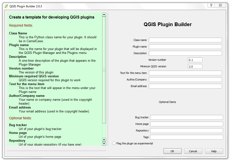
First, there are several tutorials on the web but I would start with this one.  To start, in QGIS navigate to the "Plugins" tab and download the Plugin Builder, if you don't have it installed already. The plugin builder creates a template with important information for your plugin as well as the needed files.  Click on any of the screenshots to magnify them.

QGIS Plugin Builder 2.0.3

The text in green and the link to the tutorial explain what each of the fields mean and does for your plugin. A folder with the necessary files will be created.  Remember the file path.

The next step is to compile the plugin files.  This was the first hurdle.  Eventually, I found a post with a solution.  Double-click the OSGeo4W icon on your desktop.

1. At the command prompt, point to the folder where your plugin is located.  Example:  cd: C:/Users/yourusername/.qgis2/python/plugins/pluginname (in this example CalculateArea is the name of the plugin).  You will need to substitute the fields highlighted in red.

Point to the directory where you plugin is located.

1. Next, type: pyuic4 -o ui_pluginname.py ui_pluginname.ui and press Enter
2. Lastly, pyrcc4 -o resources.py resources.qrc and press Enter

Compiling the Resource and UI files

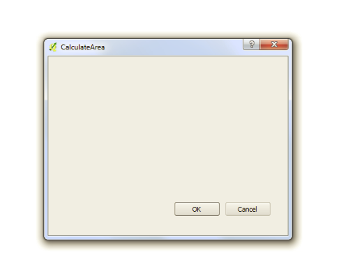
Then follow the steps for deploying and testing.  After installing the plugin from the plugin tab, you should be able to see it in the tab along with any other plugins you have installed.  Click it and the basic plugin window will appear!  You should be able to install your plugin in QGIS and see its name.

The basic plugin window with the name of your plugin

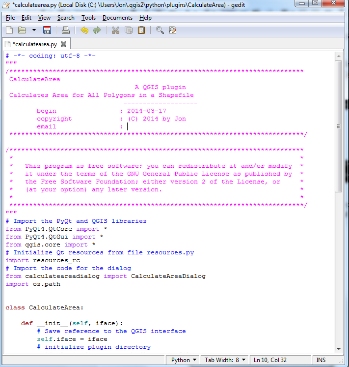
Lastly, time to start writing some python. You can download a viewer/editor like gedit.  Open up the file named pluginname.py and you will see a lot of the basic skeleton coding already written.

Viewing and editing python code from the QGIS Plugin Builder 

A few parting thoughts:  Be sure to search the QGIS repositories to see if someone has already created a plugin for what you are thinking of doing.  Borrow code from other plugins, which have been validated, to help speed the process along.

An Epic View with NASA's Worldview

In an ever-changing world, having a global view is extremely important.  NASA has developed several website/tools where you can view and download up-to-date global remote sensing data.  NASA's Worldview is one of them.  If you are looking for a quick example of its practical value, take a look at last fall's forest fires in the western U.S.

 "Most of the 100+ available products are updated within three hours of observation, essentially showing the entire Earth as it looks 'right now'. This supports time-critical application areas such as wildfire management, air quality measurements, and flood monitoring."- NASA Worldview Website

Of note, browsing on a tablet or smartphone is supported.  There is a layered slider for time, so users can choose the year, month, and day. Selecting dates in some websites can be painful.  However, this slider is intuitive, quick, and easy to use--much more so than those pesky calendar pages some users are forced to navigate.  Users also have several base maps to choose from in addition to the rest of the layers.  There is a great "About" page and brief "Tour" available.

Global Land Surface Temperatures/Day from MODIS, 17 July 2013

A few basic social features are built-in.  The website has buttons for saving links to certain views and taking screenshots.  There are lot of different instruments and views but everything is well-labeled. A few different band combinations can be selected with one-click for easy viewing.  This is especially important for looking at vegetation and agriculture, for example. 

You can also check out recent scenes from Landsat 7 at: http://earthnow.usgs.gov/ or Landsat 8 at: http://landsatlook.usgs.gov/.  If you are interested in NASA's open data policies, a quick overview can be found at: http://science.nasa.gov/earth-science/earth-science-data/data-information-policy/