R GeoNames API

R has a package (geonames) for connecting to the GeoNames API.  If you are not familiar with GeoNames be sure to check out this previous post with a few examples.  The documentation for the package can be found at: http://cran.r-project.org/web/packages/geonames/geonames.pdf

Step #1: Getting a Free Account
You will need to visit  http://www.geonames.org/login to create a free account.  Note: GeoNames has free and premium services.

Step #2: Activating the Account
After receiving a confirmation e-mail, log-in, and click the activate link.  Look midway or towards the bottom of the page.  It is easy to miss!  If you do not activate the account, you will receive an error message in R such as '401 Unauthorized'.

Step #3: Installing and Loading the Package in R
The simplest way to a install a package in R is to go the toolbar at the top, select "Install Packages", choose a download source or simply select "OK" and then scroll down until you find "geonames" in all lowercase letters.

• After the package installs, you will also have to Load Package from the same toolbar.  
• Loading the package from the toolbar will have to be done each session--unless you write a short bit of code to do the same automatically.
• Also make sure you have admin privileges on the computer you are working on.

Step #4: Connecting to the API
In R, you will have two write two lines setting "options" to access the API.  Simply replace "your username" in red with your username!  You will also have to set the host--which is currently api.geonames.org.  Please note in some older documentation and websites this is listed incorrectly as an older address.  It is also possible, although not likely, it could change in the future but would be listed here.

options(geonamesUsername="your username")

options(geonamesHost="api.geonames.org")

Step #5: Test Your Connection
In R, simply type:

source(system.file("tests","testing.R",package="geonames"),echo=TRUE)

If everything is setup correctly, R will pause for a few seconds and return geographic data like in the screenshot below.

Running the code above, you can test your connection.

Step #6: GeoNames Structure
Remember geographic data can have different hierarchies (See Place Hierarchy Webservices) and be accessed in different ways. Be sure to read through the GeoNames and R package documentation to be certain you are getting your desired result.  There are a number of user-defined functions in the GeoNames package.

Examples of user-defined functions:

• GNcities () - returns cities within a bounding box
• GNearthqukes () - returns recent earthquakes
• ...and many more!

Step #7: Getting Geographic Information from Wikipedia, Saving...
For example, one function in the package allows you search Wikipedia articles and retrieve geographic information (i.e. lat, long, elevation).  For example the following code looks for up to 10 articles with "oriole" and stores them in a R dataframe named results:

results<-GNwikipediaSearch("oriole", maxRows = 10)

Click the screenshot to open in a larger window

Example of results, with rank and geographic information, lat, long, and elevation.

You can also type "summarize(results)"--without the quotes -- remember 'results' is the name of the data set to view all of the variables.  The data can also be exported from R.  Keep in mind you can use R to perform exact or fuzzy merging with a data set of place names you have.

Review of the Spatial Computing Class on Coursera

From GPS and Google Maps to Spatial Computing was the first geospatial Coursera course that I took and my second Coursera class. Below, I describe the course, what you'll learn, and key takeaways.  Overall, the course is a unique offering that you should check out!

Overview

The eight-week course is taught by Shashi Shekar and Brent Hecht from the University of Minnesota's Department of Computer Science and Engineering.  The goal of the course is to:

"introduc[e] concepts, algorithms, programming, theory and design of spatial computing technologies such as global positioning systems (GPS), Google Maps, location-based services and geographic information systems."

The class has a workload of 4-10 hours per week depending on which of the three tracks you decide to complete (scroll to the bottom of this post to learn more about the different tracks). The majority of the weeks are close to the four hour end. Week 3's workload was heavy.  Be sure to set aside enough time to watch all of the video lectures each week.

Topics Covered

You will learn why SQL requires extensions for spatial queries as well as how to understand the results from basic spatial queries.  How spatial data are stored, accessed, and algorithms used to solve basic spatial problems (i.e. shortest-path, routing) will be discussed.

You'll also learn about volunteered geographic information, different types of positioning, and even how position can be tracked underground. There are interesting lectures about implicit and explicit spatialization--being able to visualize and analyze spatial information in different ways than you might normally think about. Lastly, you will briefly cover cartography (mainly for those new to GIS and/or computer science focused).

Course Schedule

Week 1: Introduction to Spatial Computing and Overview of Course
Week 2: Spatial Query Languages
Week 3: Spatial Networks (e.g. road networks)
Week 4: Spatial Data Mining
Week 5: Volunteered Geographic Information
Week 6: Positioning
Week 7: Cartography and Geographic Human-Computer Interaction
Week 8: Future Directions in Spatial Computing 

Platforms used: WikiBrain API and briefly TileMill

You will learn about WikiBrain - accessing data from Wikipedia and Atlasify (soon to be released).

Miscellaneous

In addition to lectures/videos and slides, you will see taped/videoconference interviews with leading geospatial professionals. In the first few weeks, I felt this worked well but got a little old as the course went on. Hopefully, future sessions will shorten the interview segments--which can be quite lengthy--and occasionally feel burdensome on top of the other coursework.  You will also have a few required readings that are directly related to the coursework and include interesting real world applications.

Tracks

• Curiosity:  come as you want! no requirements
• Concept:  Short quizzes and a Statement of Accomplishment
• Technical: Harder quizzes and assignments for a Distinguished Statement of Accomplishment
• For the Technical Track, you will need to complete quizzes for both the Concepts and Technical Track. Having programming experience is recommended for the Technical Track's programming homework.

Signature Track available: Yes.  To learn more about Coursera's signature track visit: https://www.coursera.org/signature/guidebook

You will want to sign-up now for e-mail reminders about future sessions, since Coursera offerings are typically spaced several months apart.  For other geospatial classes on Coursera, visit my earlier post: http://opensourcegisblog.blogspot.com/2014/08/free-online-mapping-classes-from-psu.html.  I will be updating this list in the months to come.  (Please note, like other Coursera classes, it will take several weeks for your Statement of Accomplishment to be posted.)

GeoNames: 8 Million-plus Placenames for Free

GeoNames is an open-source geographical database, which you can download, that contains information on many types of features, in various languages, has attribute data (such as elevation) and comes with lat/long coordinates.

You can see a breakdown of the number of features by country at: www.geonames.org/statistics/.  In addition to being able to download the data in bulk, GeoNames also has collaboration and editing features similar to other open mapping ecosystems.

Example: Populated Places Around Mt. Everest
Before downloading,  open the Readme: http://download.geonames.org/export/dump/readme.txt to make sure you are grabbing the correct files.  It will also describe the column names and send you to a few other webpages for reference information.  For example, you will also want to read through the feature codes at: http://www.geonames.org/export/codes.html

Populated places (PPL) from GeoNames.  Click to enlarge.
Other data sources: USGS (DEM) and Natural Earth (Roads, Rivers,etc.).

There are also free and premium web services: http://www.geonames.org/commercial-webservices.html

Editing

GeoNames also allows users to add and edit data.  A screenshot of the interface for Mt. Everest:

Add/Edit Interface

You can also view a history of edits:

Wikipedia Map

Lastly, you can even view Wikipedia entries on an interactive map:

Markers pop-up for entries in Wikipedia

GeoNames data sources: http://www.geonames.org/data-sources.html

QGIS on Raspberry Pi

Raspberry Pi is a low-cost credit-card sized computer that has gained notoriety for programming, education, and a wide variety of other projects. In this post, I will talk about using QGIS with Raspberry Pi as hardware.

I will cover the different models for Raspberry Pi, which one you should use, other accessories, installing an operating system (OS), and more!  If you have any suggestions, please let me know in the comments section below.

Where to purchase
Raspberry Pi can be purchased online through Amazon.com and other online retailers.  Some specialty electronic stores, like Micro Center, and hobby shops also carry it in stock.  Expect to pay more in physical stores than online.  Also, it can be easier to find accessories online than in brick and mortar stores, where I had to hunt through bins!

What to purchase
There are two models of the Raspberry Pi: Model B+, the newest version, and Model B.  Model B+ carries a number of significant improvements over Model B including: More USB ports (4 vs 2), Micro SD slot for storage, lower power consumption, and better audio.  Both models also sport an HDMI connection.  The Model B+ is also organized better with an improved layout.  Both models sport the same processor and 512 MB of RAM.

Comparison of Model B+ and Model B, Raspberry Pi

I purchased a Raspberry Pi Model B+ Starter Kit ($60 USD/48 Euros/6739 Yen) since it contains nearly everything you need to get started including a case to protect your device, power supply, Micro SD card with SD adapter (several OS already installed), and a brief user's guide.  (Note: the Micro SD card needs to be removed to completely close the case).

Additional Items
I purchased an inexpensive card reader to be able to copy files from my computer onto the Micro SD card that I will use in the Raspberry Pi. I also got a Samsung micro SD card PRO with a larger capacity (16 GB), faster read speeds up to 90 MB per second, and write speeds of 50 MB per second ($20 USD/ 6 Euros /2246 Yen).

Lastly, I purchased a Wi-Pi, a wireless adapter ($14 USD/11 Euros/1572 Yen) designed for the Raspberry Pi.  Already on hand, I have a regular sized keyboard and mouse, a monitor (or TV can be used), an array of cables (USB and HDMI) and as an alternate: a small wireless keyboard with mouse pad.

Instructions
There are several posts on installing QGIS on Raspberry Pi including one on StackExchange.

Sources of Frustration
Minor: The Raspberry Pi may not detect your monitor or TV size and resolution at first.  You can also edit a config file to match your desired characteristics.

Major: I had issues with Debian, upgrading from Wheezy to Jessie, and being able to re-boot.  From Goggling, the issues I had are known - and not new.

Success or Failure?
I was able to install QGIS on the Raspberry, see below for a screenshot, but it is slow. I was also able to install plugins.

Success but was it worth it?

Worth the Effort?
It will take at least 2-3 hours to go from Wheezy to Jessie and install QGIS.  Expect to spend more time, if like me, you are new to Linux-based systems, you run into difficulties, or need to start from scratch.  For the moment, I won't be using my Raspberry Pi for GIS, but I may check-back in on it later.  I think I will be using the Raspberry for its more typical uses.

Customizing Qgis2threejs Code

I have received a few e-mails about customizing the output from the cool Qgis2threejs plugin, created by Minoru Akagi.  The QGIS plugin allows for the creation of a 3D map that can be placed in a website or run off your computer's web browser, without having to install any additional software.

The plugin has been improved and enhanced since my original post on Manhattan and follow-up post.  The best part is that the code is well annotated and easy to follow, so you do not need to be a coding expert to make some neat and fun changes!

In this post, I open up a few of the different file types, edit a few values, and show the results.  I will also briefly talk about some of the plugins newer options, including labels!  What mapper does not love to be able to add labels...and labels for 3D!  Neat stuff!!

Saving the Plugin's Output

At the bottom of the plugin, you will see a white box that allows you to browse to a location to store the output.  Selecting a location, several files will be output instead of being stored in a temporary folder.

Results are easy to export to a folder destination of your choosing.

Starting view: Before changing the code

Starting view from the plugin (before any changes to code)

HTML File:  Camera and Controls

First, I will edit the starting position of the camera.  The three values for the camera.position.set are X,Y, and Z values.

Original:

 var camera = new THREE.PerspectiveCamera(45, width / height, 0.1, 1000);

  camera.position.set(0, -100, 100);

Changed to:

 var camera = new THREE.PerspectiveCamera(45, width / height, 0.1, 1000);

  camera.position.set(0, 0, 75);

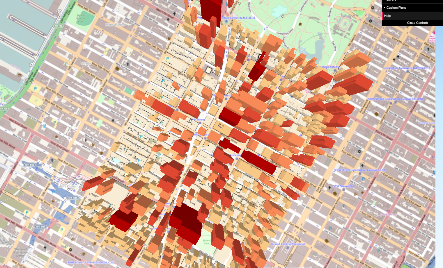
Result from changing the camera position - now overhead view and close-up.

Qgis2threejs.css: Changing the starting background gradient

Many websites will tell you the color codes to build a new color gradient.  Here, I changed the nice default blue gradient to a burnt orange sky.

Original:

#webgl { background: linear-gradient(to bottom, #98c8f6 0%,#cbebff 40%,#f0f9ff 100%); }

Changed to:

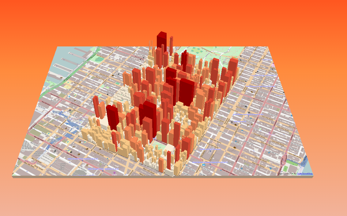
#webgl { background: linear-gradient(to bottom, #FF350D 0%,#FF8B3D 40%,#EFBBAE 100%); }

Changing the starting background color is easy to do too!

Within QGIS and the plugin, there are a few basic background options as well, such as making it a solid color.

Additional new features

A number of improvements have been made to the plugin, which is also easier to use.  You can add multiple types of GIS files.  You can also label attributes on your 3D map, although there is a cost to performance.  Labeling lots of features will grind your map to a halt.

Labels can be added now, in this case roof heights

An Introduction to Leaflet, Part III: Comparing Heatmap Plugins

A great advantage and disadvantage of free and open source GIS (FOSS GIS) is the variety of options out there.  In this post, we will take a look at four different heatmap plugins for Leaflet.  If you want to skip to the final product, visit: http://webmapexamples.net/leaflet/heatmap/heatcompare.html
to see the final comparison.

We will take a look at four different plugins listed on Leaflet's plugin page:

• Heatmap.js
• HeatCanvas
• Leaflet-div-heatmap
• WebGL Heatmap

Screenshot of the comparison site: http://webmapexamples.net/leaflet/heatmap/heatcompare.html

Data
I used QGIS to generate 500 random points within the state of New Hampshire.

Each plugin references point data and intensity/weight values in slightly different way.  For the three plugins I got to work, here are how points should be formatted.

• Heatmap.js: [{lat: , lng: , count: },...
• HeatCanvas: [0,0, 1] point at 0,0 with count 1
• Leaflet-div-heatmap: [{lat: , long: , value: },...
• WebGL Heatmap: N/A

Overall Impressions

Performance: Heatmap.js was fastest. (Although I did not have a chance to use WebGL Heatmap.  HeatCanvas was slowest rendering.

Ease of Use: Heatmap.js was the clear winner! Leaflet-div-heatmap required more knowledge of JavaScript and I ended up editing the actual plugin code.  WebGL required understanding that!

Documentation: Heatmap.js and HeatCanvas were good.  For Heatmap js be sure to visit the website separate from github.  Leaflet-div-heatmap had poor documentation.

Other considerations: I couldn't quite get the WebGL plugin to work - when adding point data. However, I was able to get a demo working and be able to interactively change density using my mouse with another *.html file.  However, WebGL does boast performance for large datasets, so I may return to it a later date.  The Leaflet-div-heatmap uses sort of collect events/morph feature, so it is different from the rest, be sure to zoom in on the map.  This will become clearer when you try it... Also don't forget to check out each plugin and their array of options!

Heatmap Comparison webpage:
http://webmapexamples.net/leaflet/heatmap/heatcompare.html

See also:
Leaflet.heat
SimpleHeat
Leanpub: Leaflet Tips and Tricks
A related post in Stackoverflow

An Introduction to Leaflet, Part II: Adding GeoJSON from an External File

Last time, I wrote about adding data from a spreadsheet.  In today's post, I will show how to load GeoJSON data from an external file and create a legend with mutually exclusive categories.

In many tutorials, GeoJSON data is incorporated as part of the code.  However, with a large number of features comes a large block of code that can make writing and debugging difficult. So, reading in the data straight from an external file is valuable.  (One method that is not recommended is creating a JavaScript variable in the GeoJSON file.)

I will be condensing a longer blog post by Lyzi Diamond but feel free to head over to her page for the full explanation and the complete details.  I will also be using code from the Leaflet chloropleth map tutorial, and give its legend a needed update.

The Data
For this post, I will be creating a map of health insurance rates  (2012) in Texas based on data gathered for a post earlier this year on health insurance rates.

What You Will Need
You will need jQuery, a JavaScript library that makes life easier.

Loading the GeoJSON file
In the head of the document, in between style tags, load the jQuery script and reference the GeoJSON file using a link relation.  Here, the file is texas2.geojson.

<script src="./jquery.min.js"></script>
<link rel="polygon" type="application/json" href="/leaflet/healthinsurance/texas2.geojson">    

...and in the body...

$.getJSON($('link[rel="polygon"]').attr("href"), function(data){
var geojson = L.geoJson(data,{...
                .,,with additional code for styling and the popup.

Styling
The Leaflet chloropleth tutorial has nice code for styling by creating two JavaScript functions and using ColorBrewer for getting colors in hexadecimal.

The Legend
The legend code from the Leaflet tutorial is really neat but it needs a little updating.  The legend's categories are not mutually exclusive.  So, I created two arrays (one for the lower bound, the other for upper bound of the categories for percent uninsured) instead of just one for the lower bound in the tutorial.

  var div = L.DomUtil.create('div', 'info legend'),
        lower = [2,12.6,16.9,21,26],
        upper = [12.5,16.8,20.9,25.9,"plus"],
        labels = [];

    // loop through our density intervals and generate a label with a colored square for each interval
    for (var i = 0; i < lower.length; i++) {
        div.innerHTML +=
            '<i style="background:' + getColor(lower[i] + 1) + '"></i> ' +
            lower[i] + '&ndash;' + upper[i]+'<br>';
   }
    return div;
};

I've updated Leaflet's code to make a mutually exclusive legend.

The Final Map
The final map can be viewed at: http://webmapexamples.net/leaflet/healthinsurance/Texas.html. Don't forget,on the webpage you can right-click with your mouse and select "view source" to see the final code.

The final map has popups for County Name + Percent Uninsured

I am still deciding on the topic for the next Leaflet post.  If you have any suggestions, please leave them in the comment section below.