Spatial Analysis with GeoDa: Part II - Importing Data and Tools

GeoDa opens as a "floating bar" which you will find nice as you do analysis and realize multiple linked windows can be arranged.  The maps and graphs are interactive, as I'll show in later posts, show selecting features in one window will highlight the same parts in other windows.

When I learn a new piece of software, I always go from left to right.  

File Menu
The "File" menu allows you to import data, save and load projects (self-named *.gda files), and export selected data. In addition, there is a nice Project Information option that tells the title, data source and type, project name, number of observations and fields.

Data Formats
Users can import a wide array of file formats: shapefile, SQLite/SpatialLite, *.csv , .xls, .dbf, .json, .gml, .kml, and MapInfo files.  Remember, are analyzing vector data, so points, lines, and polygons. Remember map projections matter, since spatial weights are created based on distance!

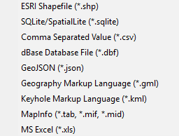
GeoDa does a great job of offering multiple file types to import.

Tools Menu: Spatial Weights
Spatial weights are used to model spatial relationships. Using GeoDa, we can create spatial weights based on contiguity/bordering (think chess moves: rook or queen), distance, and the number of nearest neighbors.  Imagine a grid or matrix that has a row and column for every feature.  The cells are populated using 0/1 for weights based on contiguity (where a feature borders another) or distances for distanced based weights.

Tips:

• Generally, do not go above 2nd order of contiguity: 1st order contiguity is neighbors, 2nd order is neighbors of neighbors.  Anything beyond this becomes extremely difficult to interpret.
• The GeoDa Center also has PySAL an open source Python library that can be used to create spatial weights and perform spatial analysis.

The first option is "Select" if you have already created weights.  The second option is "Create."  Here you will a couple of options to examiner spatial relationships in your data.  Which one you choose should be based on the phenomenon you are studying. Like other types of analysis, you will also want to examine how different spatial weights affect your results.

• More about contiguity based spatial weights: https://geodacenter.asu.edu/node/380 and distance-based weights: https://geodacenter.asu.edu/node/384

Connectivity Histogram
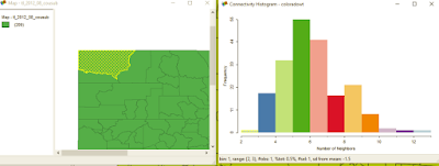
Another one of GeoDa's cool features is a histogram that shows the number of features with a specific number of features.  It can also help you clear up any questions you have about different types of contiguity and how spatial relationships are modeled.

On the histogram a right, the bar/bin for two neighbors is selected.
On the map at left the county is highlighted. Selecting other bars would highlight more features.
Users can also see the distribution of the spatial weights from the histogram.

Shape
In case you tabular data, you can create points from this menu. You can also create a bounding box or grid.  Next time, we'll look at the Table and Map toolbars.

Want blog or YouTube updates?  You can follow me @jontheepi: https://twitter.com/jontheepi

An Introduction to Leaflet, Part II: Adding GeoJSON from an External File

Last time, I wrote about adding data from a spreadsheet.  In today's post, I will show how to load GeoJSON data from an external file and create a legend with mutually exclusive categories.

In many tutorials, GeoJSON data is incorporated as part of the code.  However, with a large number of features comes a large block of code that can make writing and debugging difficult. So, reading in the data straight from an external file is valuable.  (One method that is not recommended is creating a JavaScript variable in the GeoJSON file.)

I will be condensing a longer blog post by Lyzi Diamond but feel free to head over to her page for the full explanation and the complete details.  I will also be using code from the Leaflet chloropleth map tutorial, and give its legend a needed update.

The Data
For this post, I will be creating a map of health insurance rates  (2012) in Texas based on data gathered for a post earlier this year on health insurance rates.

What You Will Need
You will need jQuery, a JavaScript library that makes life easier.

Loading the GeoJSON file
In the head of the document, in between style tags, load the jQuery script and reference the GeoJSON file using a link relation.  Here, the file is texas2.geojson.

<script src="./jquery.min.js"></script>
<link rel="polygon" type="application/json" href="/leaflet/healthinsurance/texas2.geojson">    

...and in the body...

$.getJSON($('link[rel="polygon"]').attr("href"), function(data){
var geojson = L.geoJson(data,{...
                .,,with additional code for styling and the popup.

Styling
The Leaflet chloropleth tutorial has nice code for styling by creating two JavaScript functions and using ColorBrewer for getting colors in hexadecimal.

The Legend
The legend code from the Leaflet tutorial is really neat but it needs a little updating.  The legend's categories are not mutually exclusive.  So, I created two arrays (one for the lower bound, the other for upper bound of the categories for percent uninsured) instead of just one for the lower bound in the tutorial.

  var div = L.DomUtil.create('div', 'info legend'),
        lower = [2,12.6,16.9,21,26],
        upper = [12.5,16.8,20.9,25.9,"plus"],
        labels = [];

    // loop through our density intervals and generate a label with a colored square for each interval
    for (var i = 0; i < lower.length; i++) {
        div.innerHTML +=
            '<i style="background:' + getColor(lower[i] + 1) + '"></i> ' +
            lower[i] + '&ndash;' + upper[i]+'<br>';
   }
    return div;
};

I've updated Leaflet's code to make a mutually exclusive legend.

The Final Map
The final map can be viewed at: http://webmapexamples.net/leaflet/healthinsurance/Texas.html. Don't forget,on the webpage you can right-click with your mouse and select "view source" to see the final code.

The final map has popups for County Name + Percent Uninsured

I am still deciding on the topic for the next Leaflet post.  If you have any suggestions, please leave them in the comment section below.