Healthcare Worker Deaths from Coronavirus (COVID-19): Update - 71 deaths, CDC Study

As of 4/15, 71 healthcare workers have died of coronavirus (COVID-19) in the US. Updated numbers at: https://jontheepi.shinyapps.io/hcwcoronavirus/.

• Roughly half of deaths occurred among Nurses and Certified Nursing Assistants
• Median age = 56 years old, range 20 - 75 years old
• Most have occurred in Hospitals. Of note, VA hospitals have had 8 COVID-related deaths
• New York State (13), Michigan (8), New Jersey (8), and Florida (7) are the states with most healthcare worker fatalities

The code and data for this project are available on GitHub: https://github.com/jontheepi/hcwcoronavirus

The CDC has published a study and found only 27-related deaths, highlighting shortcomings in recording deaths and occupation, and recording the impact of COVID-19 on healthcare workers:https://www.cdc.gov/mmwr/volumes/69/wr/mm6915e6.htm?s_cid=mm6915e6_x.

Healthcare worker deaths in the US from novel Coronavirus (COVID-19)

Created a quick app based on news reports: https://jontheepi.shinyapps.io/hcwcoronavirus/.

• Eight-related deaths so far. I hope not to have to update this. 
• Healthcare workers will make up a disproportionate percent of cases and possibly also fatalities. 
• The app was created using R, rshiny(package), and shinyapps.io for hosting
• Map will be updated daily.
• China only reported 5 deaths in healthcare workers. Healthcare personnel made up 4% of cases. Fifteen percent of healthcare workers that got ill were classified as severe cases. (https://jamanetwork.com/journals/jama/fullarticle/2762130)

Book Review: An Introduction to R for Spatial Analysis and Mapping

I decided to talk a walk on the wild-side and examined R as a GIS for spatial analysis.  I hope to use several of R's spatial statistics packages and to automate tasks--staying within one program.  I highly recommend Brunsdon and Comber's book ($50 on Amazon, Paperback, electronic versions also available).

About the Authors: Chris Brunsdon is the creator of geographically weighted regression or GWR. Lex Comber is a professor at Leeds University.

Four Reasons to choose R as a GIS
1)  You are interested in performing tailored exploratory spatial data analysis (ESDA), spatial statistics, regression analysis, and diagnostics.

• Of course, R is also way better than ArcGIS and QGIS for summary statistics too. (Notably, QGIS has integrated a R processing toolbox into it. ArcGIS  also has an official bridge to R.)

2)  You already use R for non-spatial data, have lots of code written, and need to analyze spatial data.

3)  You do not want to export your data (or results) from one program into another and back again!

4) You want to be able to publish or share your code with a wider audience.

A great cover to a great book!

Reader Accessibility
The content is extremely well-presented, clear and concise, and includes color graphics. It is not overly technical. Still, R as a GIS and spatial analysis are tough material and is definitely not for the faint-of-heart. The authors assume readers may not have either a R or GIS background, or both. I took a R class in graduate school and occasionally use it.

Additional packages that assist in manipulating and reshaping data, such as plyr, are also discussed. The authors also warn readers that R packages can change over time, causing error messages, but many warn users about recent and upcoming changes.

Overview
In the first 40 pages, you will learn R basics, if you don't already have a foundation. Next, you will learn GIS fundamentals, how to plot data to create a map, taking into account scale, and adding and positioning common map elements like a north arrow and scale bar. This may sound basic but in R nothing is easy!  Of course, the advantage with code is that you can reuse it or may only need to modify it slightly for many maps.

Late in Chapter 5-6 the book dives into spatial analysis.  The last few chapters are probably the best of the book, as more advanced statistical techniques are discussed including local indicators of spatial auto correlation (LISAs), geographically weighted summary statistics and regression.

The book providers a great guide and reference, and I am sure I will be re-visiting it frequently!  Overall, it is a great mix of practice and theory.

Disclosures: 
None, I found and purchased the book on my own.

Repost: R's twitteR and Accessing the 1 Percent of Geotagged Tweet

About 1 percent of all tweets are geotagged.  Fortunately, most of these geotagged tweets fall into public stream data.

Of course, this only applies to Twitter.  The percent of geotagged media varies by social network source.  For example, Instagram had up to 25% of photos geotagged by users in 2012, according to the New York Times.

We will take a look at the twitteR package in R that provides an interface with the Twitter API. The main reason I chose this was my familiarity with R.

Getting a Twitter Dev Account
First, head over to https://apps.twitter.com/.  You can use your regular Twitter account to login. Click on the "Create New App" button in the upper right-hand corner.  Follow the on-screen instructions and be sure to read the Developer Agreement.

After your "app" is created, click on the "Permissions" tab and make sure the last radio button is selected: "Read, Write, and Access direct messages."  Also check out the Keys and Access Token, especially if you are more familiar with connecting to APIs.

Connecting with R
For this blog, I am using R 3.1.3 64-bit.  Start R, then follow the instructions located in the screenshot below. Click the screenshot for a closer look.

Click the above screenshot to get a closer look.

Update #1 12/10/2015:
In addition to the code listed above, you will have to install one additional package:
install.packages('base64enc')

Otherwise, you will oauth errors.

Concluding remarks...
Connecting to and using an API may not be your strong suit, but it is not mine either!  Hopefully, I've saved you some time and got you connected to this valuable source of data!

You can also now follow me on Twitter at: @jontheepi.  I will post blog updates there as well as additional quick insights about open source GIS and mapping.

Spatial Analysis with QGIS - Part I: Point Data

QGIS 2.8 Wien was released, so it is a good time to review QGIS's basic spatial analysis capabilities for vector data--starting with point data. We will also take a look at a few plugins and the SAGA and R processing toolboxes. Most of the functionality in QGIS is from Ftools, formerly a plugin, now part of base QGIS. There is also the MMQGIS plugin to examine vector data.

In addition, I will make a few recommendations for added features, or point you to another free or open source program that can be used in conjunction with QGIS or simply by importing and exporting data.

Nearest Neighbor Index

QGIS can calculate the nearest neighbor index to assess point clustering.  No p-value is given but the simple trick is to remember that large negative z-scores mean the points are clustered while large positive z-scores mean the data is more dispersed.

No p-values are given but remembering critical values/decision points,i.e. +/-1.65, 1.96,
is the easiest way to know if clustering is statistically significant.

Mean Center and Standard Distance
The mean center, an average of x- and y- coordinates, is an easy way to find the central feature and to examine spatial-temporal trends.  In the case below, the mean of all starting points, by year, for US tornadoes, 2000-2013. The data are grouped by UID, in this case a year variable.  It would be great to also be able to calculate a median center.  Data source: NOAA Storm Prediction Center.

• In some years, the average was pulled slightly west or east.  Interestingly, the mean is pulled east in 2011, when there was a large 'outbreak' of tornadoes across the southeastern US.

The mean of all 'starting' points for US tornadoes, by year, 2000-2013.

Moreover, there are several point pattern analysis tools, including the standard distance--a measure of dispersion--in the SAGA Processing Toolbox.  More specifically the "Geostatistics" tool, contains a lot of useful functions that can be used.  The output can be  saved and displayed in QGIS.  The NOAA dataset already contains the length from start to end, but you could also calculate this by creating a distance matrix in QGIS.

The SAGA Geostatistics Toolbox in QGIS

Ripley's K
Ripley's K helps to determine clustering at different distances.  It can be implemented through the R processing toolbox in QGIS, using R's SpatStat package, or CrimeStat.

Heatmap
You can download the Heatmap plugin or use a built-in live/dynamic heat map when you go to style a layer.  For the latter, make sure to move the rendering slider to 'best' for a nice looking heatmap. Here is an example using the dynamic heat map to look at homicides in Philadelphia. Data source: OpenDataPhilly.   In future posts, we will also look at alternatives to heatmaps, like gridding/quadrat analysis.

QGIS has lot of neat options for styling vector data, including a dynamic heatmap
that changes as you zoom in and out.

 (Note: In ArcGIS kernel density tool (not to be confused with point density) remains separate from the base software and has to be purchased through the Spatial Analyst Extension).

Grouping Analysis
Lastly, grouping analysis can be examined using PostGIS, which allows for a wide variety of spatial queries using SQL, or CrimeStat.

Near future...
We will look at spatial analysis of line and polygon data as well joining points for analysis.

GME and ArcGIS
When using ArcGIS, be sure to check out the free windows-based program Geospatial Modelling Environment, or GME formerly 'Hawth's Tools," http://www.spatialecology.com/gme/.  GME has a long list of helpeful commands: http://www.spatialecology.com/gme/gmecommands.htm.

SaTScan 9.4 released, better than ever!

SaTScan is a program for detecting clusters over space, time, and space-time.  It is available for Windows, Mac OS X, and Linux. SaTScan 9.4 was recently released and it is better than ever!  The data import wizard now allows shapefiles to be read and and a graphing feature has been added to help examine temporal trends. Visit the link for a better look at the rundown of new features.

The Import Wizard now reads shapefiles.

In previous posts, I've covered the types of files you will need and how to aggregate data in preparation for importing it. Since version 9.2, SaTScan has had the ability to export *.kml and *.shp so that the most likely clusters can be viewed in GIS software. (Aside: Google Earth Pro is now free! https://www.google.com/work/mapsearth/products/earthpro.html)

Below is an example looking at clusters of low immunization rates in California from the journal Pediatrics. Free full-text: http://pediatrics.aappublications.org/content/135/2/280.full.pdf+html

In SaTScan, using lat/long coordinates, allows users to export to *.kml and *.shp.
Google Earth opens the *.kml automatically when a run is complete.

A few tutorials are being made, http://www.satscan.org/tutorials.html and sample data is available. Be sure to read the expertly written user's guide before running: http://goo.gl/rHg7M6. and the long and varied bibliography of analyses conducted with SaTScan: http://www.satscan.org/references.html

Update #1 (2/20/15)
Scan statistics can also be implemented in R's Spatial Epi Package and rsatscan.

Using R to Prepare a Case File for SatScan

SaTScan requires several different types of files for analysis: 1)  A case file with a column for the geographic unit. day, month or year (see documentation), and number of cases.  You can aggregate the data into any geographic unit--large or small. 2) A geographic coordinate file (cartesian or lat/long) with the name of the unit (i.e. census tract), x and y for centroids of the geographic units, and 3) population file with the estimated population over the time period-- by year.

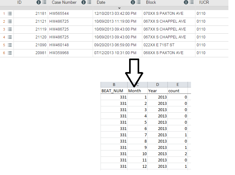
In this post, I will describe creating a case file using code in R.  The goal is to create a sum of homicides by month, year (just 2013 for this example), and police beat/post.  We won't worry about any other specifics (i.e. degree) or related types of crimes, i.e. shootings.

To ready yourself for data preparation, read Richard Block's tutorial or the more extensive SatScan manual.

I use crime data from Chicago's Open Data Portal.  The same code can be applied to other types of data, health data, etc.  A few key points: 1) the data contains victim-based data--which we want to convert into incidents. 2) not every post has a homicide, and 3) the reference post list contains 275 post.  So, we will end up with a data set with 3300 rows (275 x 12 months) or simply a row for each post-month.

If you want to skip ahead and just look at the code, go to: http://goo.gl/pmOi1u.

At the top: What you start with.  Bottom: After processing in R

Overview of Steps: See the code for further details

Step #1: Two files are imported: 1) a victim-based file of all crimes, which is narrowed down to just homicides (you could also add in shootings) and 2) a 'reference' file or simply a list of the police beats/posts in Chicago.

Step #2:  The data are summed up so that each row contains the total number of victims, then grouped again into incidents by using two different count variables.

Step #3: The list of police beats get column variables for each month in the year and expanded by reshaping data from wide to long.  This serves as a 'reference list' for matching purposes.

Step #4:  The two data sets are matched the 'unmatched' records are also kept.  These are post-months that don't have a homicide, so each count value is replaced with a zero.

Step #5: To ensure the code has worked, I check the total number of rows (3300) and spot check various posts to make sure the data has been grouped in to incidents and posts correctly.  

Whether in R or using for-fee software (i.e. SAS, STATA), preparing data for SaTScan is relatively straightforward but there are a number of steps.

Update #1 (2/18/15)
Scan statistics can also be implemented in R's Spatial Epi Package and rsatscan .

FGBASE: Fast Grid-Based Spatial Data Mining

FGBASE is a new open source software for using scan statistics on gridded data.  Unlike SaTScan, FGBASE only currently runs on Mac OS X (10.6, 10.7, and 10.8) instead of Windows and also allows for its source code to be downloaded here: http://www.fgbase.org/download-fgbase/.  The software was specifically created for environmental epidemiology but has potential applications to any fields of study concerned with finding clusters.

Analyzing aggregate data, using either software package, helps to speed up computationally intensive equations for finding spatial, temporal, or spatiotemporal clusters.

Comparison of FGBASE and SaTScan

	FGBASE	SaTScan
Operating system(s)	Mac OS X	Windows, Linux, Mac OS X
Open source code	Yes	No
Geographic output	In app	New: Export to KML or SHP
Sample data sets	Yes, 1	Yes, several
Documentation	TBD	Extensive
Publications	1	Extensive, hundreds

           

Although FGBASE comes with some sample data (available at: http://www.fgbase.org/user-data/), the program was only recently released.  Aside: The data set is different from the one used in the published paper, so you will notice differences when looking at your screen.  What data sets you will need and how they are structured is available at: http://www.fgbase.org/user-data/.

Clusters can be examined using a data-driven approach answering the question: where are the clusters?  Or, a hypothesis-driven approach can be used: are there clusters relative to a source(s) of exposure, where entities (factories,etc.) may be responsible for the clustering of cases.

A stock screenshot of FGBASE. Source: IJHG

I downloaded and installed FGBASE.  I will check back in with more impressions in a few months. Adding documentation, with a tutorial, or even a short YouTube video could greatly aid users.  I also plan to blog about getting data into SatScan and interpreting results later in the year.  Since FGBASE's source code is public, hopefully this will speed further development of the program and aid troubleshooting.

Read more at the International Journal of Health Geographics:
http://www.ij-healthgeographics.com/content/pdf/1476-072X-13-46.pdf

See also:
Treescan
R: Spatial Epi Package
There is also an experimental SaTSViz plugin in QGIS but I have not had a chance to look at.

R GeoNames API

R has a package (geonames) for connecting to the GeoNames API.  If you are not familiar with GeoNames be sure to check out this previous post with a few examples.  The documentation for the package can be found at: http://cran.r-project.org/web/packages/geonames/geonames.pdf

Step #1: Getting a Free Account
You will need to visit  http://www.geonames.org/login to create a free account.  Note: GeoNames has free and premium services.

Step #2: Activating the Account
After receiving a confirmation e-mail, log-in, and click the activate link.  Look midway or towards the bottom of the page.  It is easy to miss!  If you do not activate the account, you will receive an error message in R such as '401 Unauthorized'.

Step #3: Installing and Loading the Package in R
The simplest way to a install a package in R is to go the toolbar at the top, select "Install Packages", choose a download source or simply select "OK" and then scroll down until you find "geonames" in all lowercase letters.

• After the package installs, you will also have to Load Package from the same toolbar.  
• Loading the package from the toolbar will have to be done each session--unless you write a short bit of code to do the same automatically.
• Also make sure you have admin privileges on the computer you are working on.

Step #4: Connecting to the API
In R, you will have two write two lines setting "options" to access the API.  Simply replace "your username" in red with your username!  You will also have to set the host--which is currently api.geonames.org.  Please note in some older documentation and websites this is listed incorrectly as an older address.  It is also possible, although not likely, it could change in the future but would be listed here.

options(geonamesUsername="your username")

options(geonamesHost="api.geonames.org")

Step #5: Test Your Connection
In R, simply type:

source(system.file("tests","testing.R",package="geonames"),echo=TRUE)

If everything is setup correctly, R will pause for a few seconds and return geographic data like in the screenshot below.

Running the code above, you can test your connection.

Step #6: GeoNames Structure
Remember geographic data can have different hierarchies (See Place Hierarchy Webservices) and be accessed in different ways. Be sure to read through the GeoNames and R package documentation to be certain you are getting your desired result.  There are a number of user-defined functions in the GeoNames package.

Examples of user-defined functions:

• GNcities () - returns cities within a bounding box
• GNearthqukes () - returns recent earthquakes
• ...and many more!

Step #7: Getting Geographic Information from Wikipedia, Saving...
For example, one function in the package allows you search Wikipedia articles and retrieve geographic information (i.e. lat, long, elevation).  For example the following code looks for up to 10 articles with "oriole" and stores them in a R dataframe named results:

results<-GNwikipediaSearch("oriole", maxRows = 10)

Click the screenshot to open in a larger window

Example of results, with rank and geographic information, lat, long, and elevation.

You can also type "summarize(results)"--without the quotes -- remember 'results' is the name of the data set to view all of the variables.  The data can also be exported from R.  Keep in mind you can use R to perform exact or fuzzy merging with a data set of place names you have.

Happy New Year!...What's Ahead This Year...

What can you look forward to from the Open Source GIS Blog--in the year ahead?  Well I hope to get the New Year off to a good start by finishing some R code for cleaning messy address fields. 

Most importantly, I will be featuring more ArcGIS vs. Open Source GIS "showdowns/throw downs"--comparing similar features in paid vs. free and open source GIS software, focusing on spatial analysis and other features.  These are one of my favorite posts to write but usually take the most time to create.  Here, you can check out one past post about kernel density in ArcGIS vs CrimeStat. I cannot guarantee open source GIS will win every time, but the journey will be fun!  In addition, we will be taking a look at download and using Landsat 8 data.  I also plan on posting more book reviews on books about open source GIS and other relevant topics.

Announcement:  If you are interested in Android App Development, check out the Coursera course "Programming Mobile Applications for Android Operating Systems" from the University of Maryland.  I will taking it and hope to see you there!  The course is free.  However, Coursera offers a Verified Certificate for $49--which may be worthwhile for professional development.  The course beings on January 21st, and lasts 8 weeks, so if you are interested get registered now!  Check out the video below!

I started this blog about two years ago...this will be third year!  Each year, I try to post higher quality information so stay tuned.  By the numbers, a few statistics:

• The blog has had a modest 5,700 page views since its first creation in February 2012. 
• Viewers have come from many different countries. 
• The most frequent users hail from my home county of the US, Latvia (real or bots/spam?), Germany, UK, Russia, France, Canada, Australia, China, and India.  However, many different countries have viewers including: Brazil, Portugal, and South Korea, and the list goes on! 
• There have been 56 posts - each with an important piece of information, software, analysis, web map, or links to great resources.
• By browser: 35% of page views have been in Firefox, 27% from Chrome Browsers, 23% from Internet Explorer, and the remainder from other mobile browsers.
• By operating system, most users are using Windows (74%), Mac (8%)--with reminder from Linux and mobile OS.

If there is something you would like to see on the blog, feel free to write in the comments below.  Again, happy new year!

CrimeStat & GME vs. ArcGIS: Kernel Density

Many spatial analyses begin with using kernel density in GIS.  In ArcGIS, kernel density is part of the Spatial Analyst Extension.  However, several viable alternatives exist.  For today's post, I chose two of the easiest to implement and the ones that I have had the most success with: CrimeStat and Geospatial Modeling Environment (GME), formerly known as Hawth's Tools. Note: For GME you will also have to have R installed and several spatial packages.  They are both free, so enjoy!

When using these different tools, keep in mind that there are different kernel functions. ArcGIS uses a quadratic estimation while CrimeStat and GME have several. Click on the image below to magnify it.   The maps show density analysis of Wifi spots in New York City.

I chose different kernel functions to highlight the intricacies of density analysis.  In addition, ESRI has a video on performing proper density analysis, which you should check out.

Crimestat is a lightweight program that is relatively straightforward.  GME requires more installation steps but uses a point-and-click interface to generate the density map. After installing GME and R, in GME, be sure to search and use r.setpath to link GME to R. In addition, in GME you can copy, paste, and edit code in the same window--an extremely helpful feature!

Notes: I have been rather frustrated with the kernel density implementation in GRASS and Quantum GIS--even after diving into the help pages and discussion boards.

Non-GIS Open Source, Worthy Companions

Do not look at the title twice!  Yes, this post is about non-GIS open source software.  However, these open-source programs make great companions to any analysis. 

For example, you may find the need for a traditional statistical software package. R Statistical Software can aid in importing, analyzing, and cleaning your data.  You can perform traditional statistical analyses.  There's even a spatial package, although you will better off sticking with open source GIS programs like GRASS or QGIS.  A good overview of its spatial package can be found here.

Want to examine social networks?  Then, Gephi's great!  I just analyzed my Facebook network in only a few minutes after following a tutorial.  In addition, Gephi has features and plugins to help you map geographic data. 
   
At some point you may also need Python.  Editing and organizing code, then give Notepad ++ a try.

A some point you will have to compress files, then 7-zip is a sure thing.  You may want to playback some videos or animations and VLC Player works great.

GIMP is a image maniupulation program similar to photoshop.  You can see an example of combining GIS with GIMP on a great GIS blog.

You will probably want to type up your results or make a few "PowerPoint" slides...so there's Open Office and the Libre Office implementation. If you need a standalone pdf creator, then there's PDF creator.

Lastly, if you ever want to venture away from Windows or other operating systems, there's Ubuntu--an easy installation of Linux.  Be sure the open-source or for-fee programs you want to run have a Linux version before making the switch.  Naturally, many open source programs have a Linux version but some do not.