Spatial Analysis with GeoDa: Part II - Importing Data and Tools

GeoDa opens as a "floating bar" which you will find nice as you do analysis and realize multiple linked windows can be arranged.  The maps and graphs are interactive, as I'll show in later posts, show selecting features in one window will highlight the same parts in other windows.

When I learn a new piece of software, I always go from left to right.  

File Menu
The "File" menu allows you to import data, save and load projects (self-named *.gda files), and export selected data. In addition, there is a nice Project Information option that tells the title, data source and type, project name, number of observations and fields.

Data Formats
Users can import a wide array of file formats: shapefile, SQLite/SpatialLite, *.csv , .xls, .dbf, .json, .gml, .kml, and MapInfo files.  Remember, are analyzing vector data, so points, lines, and polygons. Remember map projections matter, since spatial weights are created based on distance!

GeoDa does a great job of offering multiple file types to import.

Tools Menu: Spatial Weights
Spatial weights are used to model spatial relationships. Using GeoDa, we can create spatial weights based on contiguity/bordering (think chess moves: rook or queen), distance, and the number of nearest neighbors.  Imagine a grid or matrix that has a row and column for every feature.  The cells are populated using 0/1 for weights based on contiguity (where a feature borders another) or distances for distanced based weights.

Tips:

• Generally, do not go above 2nd order of contiguity: 1st order contiguity is neighbors, 2nd order is neighbors of neighbors.  Anything beyond this becomes extremely difficult to interpret.
• The GeoDa Center also has PySAL an open source Python library that can be used to create spatial weights and perform spatial analysis.

The first option is "Select" if you have already created weights.  The second option is "Create."  Here you will a couple of options to examiner spatial relationships in your data.  Which one you choose should be based on the phenomenon you are studying. Like other types of analysis, you will also want to examine how different spatial weights affect your results.

• More about contiguity based spatial weights: https://geodacenter.asu.edu/node/380 and distance-based weights: https://geodacenter.asu.edu/node/384

Connectivity Histogram
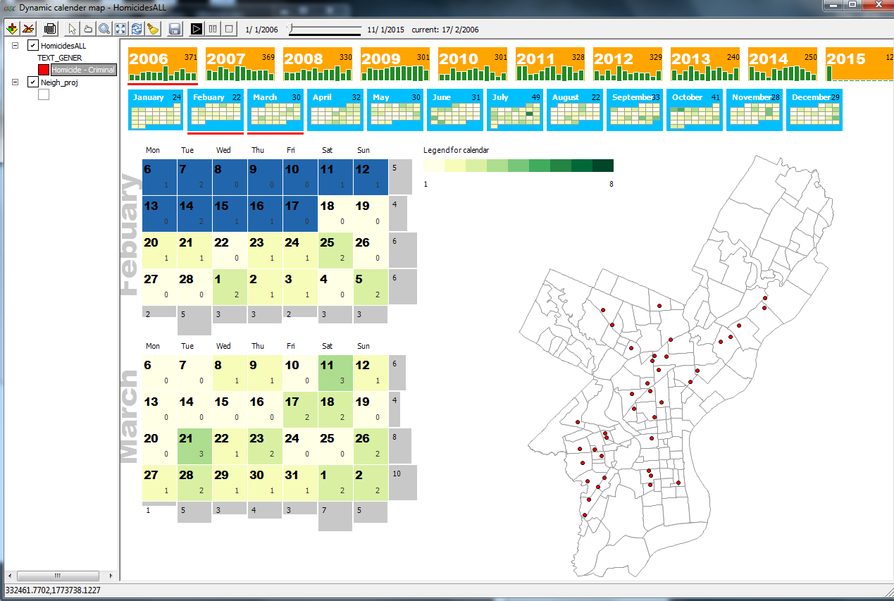
Another one of GeoDa's cool features is a histogram that shows the number of features with a specific number of features.  It can also help you clear up any questions you have about different types of contiguity and how spatial relationships are modeled.

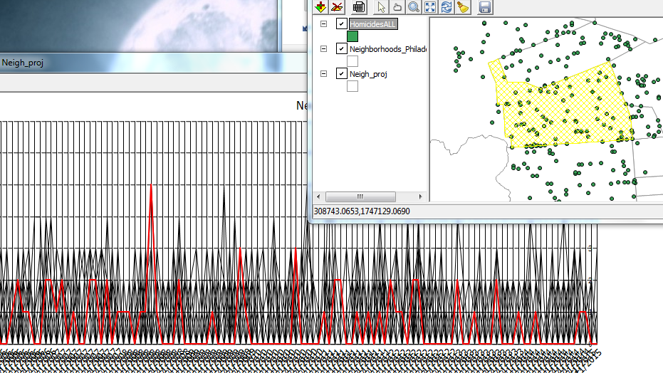
On the histogram a right, the bar/bin for two neighbors is selected.
On the map at left the county is highlighted. Selecting other bars would highlight more features.
Users can also see the distribution of the spatial weights from the histogram.

Shape
In case you tabular data, you can create points from this menu. You can also create a bounding box or grid.  Next time, we'll look at the Table and Map toolbars.

Want blog or YouTube updates?  You can follow me @jontheepi: https://twitter.com/jontheepi

Spatial Analysis with GeoDa: Part I - Introduction

GeoDa (https://geodacenter.asu.edu/software) is a free and open source cross-platform program for exploratory (spatial) data analysis or EDA/ESDA and maximum likelihood spatial regression. It has been downloaded nearly 150,000 times and is available on Windows, OS X, and Linux.  ASU's GeoDa center is home to Luc Anselin, e.g. Anselin's Moran's I a local indicator of spatial autocorrelation or LISA.

Update #1: It looks like an older version of GeoDa's source code is available (circa 2014) but not more current versions: https://code.google.com/archive/p/geoda/source

Why use GeoDa?
You are interested in spatial analysis of vector data (points, lines, polygons) and statistics.  This includes looking for clusters of count or rate data, which have similar attribute values, performing regression (asking why a certain pattern exists), observed/predicted values, residuals, and diagnostics. Spatial statistics are commonly used in mainly fields including health, criminology, and pretty much everything!

If you are using GIS for a problem, at some point, you should consider spatial statistics.  The human brain and eye can only see so much.  Some patterns aren't easily apparent.

Spatial analysis can come at a cost ($), and this is why GeoDa is so great!  It is free, open source, and has great capabilities  It even includes some advanced options which you can't currently find in ArcGIS.

Features
GeoDa includes the ability to make choropleth maps, graphs, Thiessen polygons, creating spatial weights using queen and rook contiguity (which requires a high level license in ArcGIS), graphing features by number of neighbors, linked graphs you can 'brush,' LISAs, and regression. We will dive deeper into features later--there is a lot to cover.

A list of GeoDa's features can be found at: https://geodacenter.asu.edu/general-features.  Also, here is a list of its modeling features: https://geodacenter.asu.edu/node/397.

Examples of Use

In 2014, I wrote about a simple use case: examining health insurance rates at the county-level:
http://opensourcegisblog.blogspot.com/2014/04/exploring-health-insurance-estimates-by.html.

More to come...

This is the first part in a series that explores GeoDa's functions and spatial statistics. If there is something you would like to see, leave it in the comment section below.

Want blog or YouTube updates?  You can follow me @jontheepi: https://twitter.com/jontheepi

Crime Analytics for Space-Time (CAST)

Crime Analytics for Space-Time (CAST) - alpha (2013) is a free and open-source cross-platform program (Windows, Mac OSX and Linux) designed "to detect spatial patterns and trends in crime data."

CAST is a nifty piece of software that combines key functions of other programs from the ASU GeoDA Center with a greater emphasis on temporal trends.  It even allows you to view data by calendar days, months, and years.

What you will need...
All you need is a shapefile of projected crime incident data and any boundary files (posts, census tracts, blocks, etc.).  To perform some types of cluster analysis, you will also need to aggregate your data.  If all you have is a *.csv, you can use QGIS to crate a shapefile file and save it for importing into CAST. There is sample data from San Francisco available here.

Check the format of your date field
If you are having trouble with using your data's date fields in CAST, use QGIS's field calculator to create a new variable with an output field type of "Date." Next, use "Conversions" and "to date" under the function list, and make sure the variable you enter is in the format "YYYY-MM-DD".  So, the expression should read:  todate( "Date Field" )

• Make sure to create separate fields for date and time--rather than one single field. 
• I tried a couple different formats but this format worked. 
• In CAST, you will be able to select your date field. 

CAST can do a lot!
In the "Tools" menu, you can create a grid and save it as a shapefile.  Under "Table", you can view attribute data for your shapefile. The "Weights" menu allows you to create spatial weights and view a connectivity histogram, like in GeoDA.  The "Map" menu allows you to symbolize polygons by several different criteria.  The real fun comes in the last four menus: Calendar Map, Cluster Map, Time, and Explore.

Calendar Map + Dynamic Map
One of CAST's interesting features is combing a calendar with the number of events and a map.  You can add shapefiles and layer them, although a bit tricky by clicking on each. Below are few examples using homicide data from Open Data Philly.

A calendar and map of homicides in Philadelphia starting in 2006.

Clicking a calendar will bring up a bar and pie graph (which can show a
breakdown if there is more than one category of crime/event in your data).

Graphs and maps are linked in CAST, so clicking on a feature or peak in a graph will highlight the selected features.

Like other ASU software, all graphs and maps are linked. Here one line was selected,
which represents one neighborhood, and the corresponding area on the map is highlighted.

Cluster Map
You will find a lot of tasks that are identical to GeoDA here plus some dynamic density maps.

Time & Explore
Trend graphs area available here as well as standard graphs like a histogram, scatterplot, and boxplots.

In sum...
Looking at patterns over space and time is difficult, but CAST can help.  Unfortunately, you cannot save a session in CAST so be sure to keep track of what steps you perform.  Limit your data to the time period of interest. I would not recommend adding huge point shapefiles.  Lastly, I was not able to save a movie/*.gif of animations over time, but if I figure it out, I will update this post.

For more information:
CAST Manual